SIL Simulink

SIL Simulink¶

The Veronte Autopilot 1x is implemented in Simulink blocks with an S-Function.

This kind of block takes a C, C++, Fortran or even Matlab code, and implements it in a block containing a certain number of inputs and outputs. A typical 1x Autopilot S-Function is shown below.

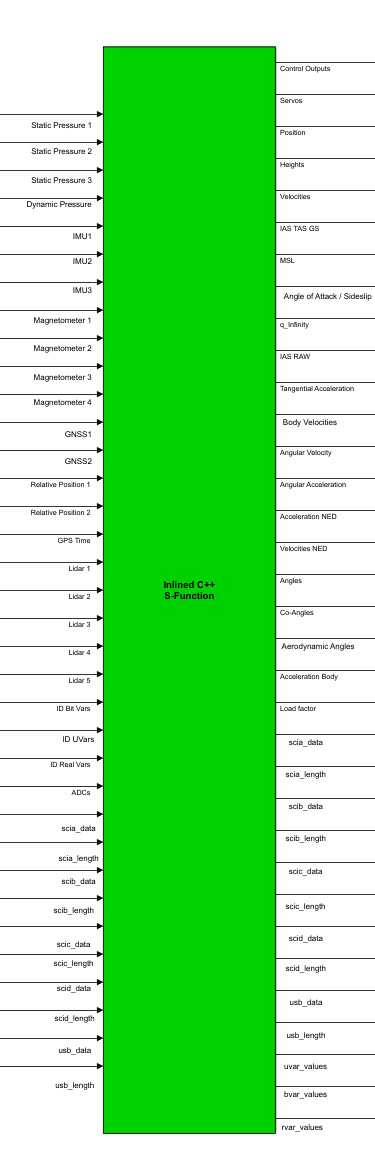
../_images/s-function.png — **S-Function containing the autopilot embedded code**¶

Inputs¶

Inputs are described in the next table:

PIN	Signal Type	Description	Form	Size	Units
1	Input	Static Pressure 1	[pressure_measurement;sensor temperature]	2x1	\(Pa\) ; \(K\)
2	Input	Static Pressure 2	[pressure_measurement;sensor temperature]	2x1	\(Pa\) ; \(K\)
3	Input	Static Pressure 3	[pressure_measurement;sensor temperature]	2x1	\(Pa\) ; \(K\)
4	Input	Dynamic Pressure	[pressure_measurement;sensor temperature]	2x1	\(Pa\) ; \(K\)
5	Input	IMU 1	[acc_x;acc_y;acc_z;gyr_x;gyr_y;gyr_z;sensor temperature]	7x1	\(\frac{m}{s^2}\) ; \(\frac{rad}{s}\) ; \(K\)
6	Input	IMU 2	[acc_x;acc_y;acc_z;gyr_x;gyr_y;gyr_z;sensor temperature]	7x1	\(\frac{m}{s^2}\) ; \(\frac{rad}{s}\) ; \(K\)
7	Input	IMU 3	[acc_x;acc_y;acc_z;gyr_x;gyr_y;gyr_z;sensor temperature]	7x1	\(\frac{m}{s^2}\) ; \(\frac{rad}{s}\) ; \(K\)
8	Input	Magnetometer 1	[mag_x;mag_y;mag_z;sensor temperature]	4x1	\(T\) ; \(K\)
9	Input	Magnetometer 2	[mag_x;mag_y;mag_z;sensor temperature]	4x1	\(T\) ; \(K\)
10	Input	Magnetometer 3	[mag_x;mag_y;mag_z;sensor temperature]	4x1	\(T\) ; \(K\)
11	Input	Magnetometer 4	[mag_x;mag_y;mag_z;sensor temperature]	4x1	\(T\) ; \(K\)
12	Input	GNSS 1	[1;3;lon;lat;alt;hr_accu;vt_accu;v_n;v_e;v_d;v_accu]	11x1	\(deg \cdot 10^7\) ; \(mm\) ; \(\frac{mm}{s}\)
13	Input	GNSS 2	[1;3;lon;lat;alt;hr_accu;vt_accu;v_n;v_e;v_d;v_accu]	11x1	\(deg \cdot 10^7\) ; \(mm\) ; \(\frac{mm}{s}\)
14	Input	Relative Position 1	[1;x_rel;y_rel;z_rel;d_x;d_y;d_z;x_accu;y_accu;z_accu]	10x1	\(cm\) ; \(mm \cdot 10^{-1}\)
15	Input	Relative Position 2	[1;x_rel;y_rel;z_rel;d_x;d_y;d_z;x_accu;y_accu;z_accu]	10x1	\(cm\) ; \(mm \cdot 10^{-1}\)
16	Input	GPS Time	[week_number;milliseconds_of_week]	2x1	-; \(ms\)
17	Input	Lidar 1	[lidar_measurement]	1x1	\(cm\)
18	Input	Lidar 2	[lidar_measurement]	1x1	\(cm\)
19	Input	Lidar 3	[lidar_measurement]	1x1	\(cm\)
20	Input	Lidar 4	[lidar_measurement]	1x1	\(cm\)
21	Input	Lidar 5	[lidar_measurement]	1x1	\(cm\)
22	Input	ID Bit Var	[Var_IDs]	50x1	-
23	Input	ID Unsigned Var	[Var_IDs]	50x1	-
24	Input	ID Real Var	[Var_IDs]	50x1	-
25	Input	ADCs	[adc(1-17)]	17x1	-
26	Input	SCIA Data	[serial_data]	1024x1	-
27	Input	SCIA Length	[serial_length]	1x1	-
28	Input	SCIB Data	[serial_data]	1024x1	-
29	Input	SCIB Length	[serial_length]	1x1	-
30	Input	SCIC Data	[serial_data]	1024x1	-
31	Input	SCIC Length	[serial_length]	1x1	-
32	Input	SCID Data	[serial_data]	1024x1	-
33	Input	SCID Length	[serial_length]	1x1	-
34	Input	USB Data	[serial_data]	1024x1	-
35	Input	USB Length	[serial_length]	1x1	-

Outputs¶

Outputs are the following:

PIN	Signal Type	Description	Form	Size	Units
1	Output	Control Outputs	[control_outputs(1-20)]	20x1	-
2	Output	Servo Values	[servos(1-32)]	32x1	-
3	Output	Position	[lon;lat;alt]	3x1	\(rad\) ; \(m\)
4	Output	Heights	[msl,agl]	2x1	\(m\)
5	Output	Velocities	[longitudinal_v;lateral_v;velocity(module)]	3x1	\(\frac{m}{s}\)
6	Output	IAS TAS GS	[ias,tas,gs]	3x1	\(\frac{m}{s}\)
7	Output	MSL	[msl_from_qnh;msl_from_ISA]	2x1	\(m\)
8	Output	Angle of Attack / Sideslip	[angle_of_attack;sideslip]	2x1	\(rad\)
9	Output	Q_Infinty	[dynamic_pressure]	1x1	\(Pa\)
10	Output	IAS RAW	[ias_raw]	1x1	\(\frac{m}{s}\)
11	Output	Tangential Acceleration	[tangential_acceleration]	1x1	\(\frac{m}{s^2}\)
12	Input	Body Velocities	[longitudinal_v;lateral_v;vertical_v]	3x1	\(\frac{m}{s}\)
13	Output	Angular Velocities	[roll_rate;pitch_rate;yaw_rate]	3x1	\(\frac{rad}{s}\)
14	Output	Angular Acceleration	[acc_z_axis;acc_y_axis;acc_x_axis]	3x1	\(\frac{rad}{s}\)
15	Output	Acceleration NED	[acc_north;acc_east;acc_down]	3x1	\(\frac{m}{s^2}\)
16	Output	Velocity NED	[v_north;v_east;v_down]	3x1	\(\frac{m}{s}\)
17	Output	Angles	[Yaw;Pitch;Roll]	3x1	\(rad\)
18	Output	Co-Angles	[co-Yaw;co-Pitch;co-Roll]	3x1	\(rad\)
19	Output	Aerodynamic Angles	[heading,flight_path;bank_angle]	3x1	\(rad\)
20	Output	Acceleration Body	[acc_x,acc_y;acc_z]	3x1	\(\frac{m}{s^2}\)
21	Output	Load factor	[nx;ny;nz]	3x1	-
22	Output	SCIA Data	[serial_data]	1024x1	-
23	Output	SCIA Length	[serial_length]	1x1	-
24	Output	SCIB Data	[serial_data]	1024x1	-
25	Output	SCIB Length	[serial_length]	1x1	-
26	Output	SCIC Data	[serial_data]	1024x1	-
27	Output	SCIC Length	[serial_length]	1x1	-
28	Output	SCID Data	[serial_data]	1024x1	-
29	Output	SCID Length	[serial_length]	1x1	-
30	Output	USB Data	[serial_data]	1024x1	-
31	Output	USB Length	[serial_length] )	1x1	-
32	Output	Unsigned Variables	[selected variables(1-50)]	50x1	-
33	Output	Bit Variables	[selected variables(1-50)]	50x1	-
34	Output	Real Variables	[selected variables(1-50)]	50x1	-

In the following sections, the user can have a look at how to implement the sensors and telemetry blocks, as well as general visualisation of a complete simulation.