SIL Simulink
A software in the loop simulation consists of a Simulink model that simulates the behaviour of the system formed by the autopilot and a vehicle, without having the physical devices connected to the computer, in contrast to the HIL which has both the autopilot and (optionally) vehicle connected to the PC. This option has several advantages when it is compared with a HIL setup:
Complete simulations without any hardware.
Possibility of using your own vehicle model: no need to stick to XPlane models. You can add as much physics/complexity as desired.
Possibility of simulating different kinds of sensors even if they are not fitted in Veronte.
All results can be exported/visualized to MATLAB workspace simultaneously.
Veronte Block runs faster than real time, allowing the user to execute a series of simulations in a short time.
Light computational load.
Autopilot Simulation
The autopilot is implemented in Simulink with an S-Function. This kind of block takes a C, C++, Fortran or even Matlab code, and implements it in a block containing a certain number of inputs and outputs. A typical Veronte s-function is shown below.
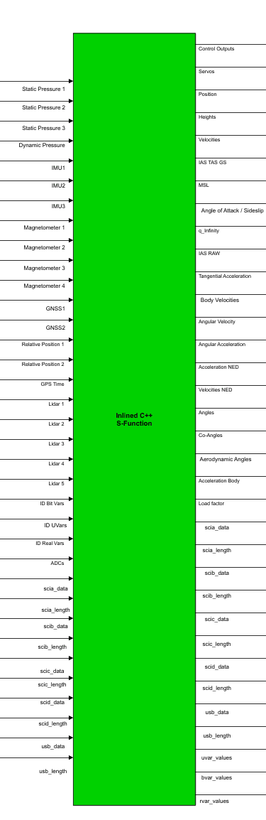
S-Function containing the autopilot embedded code
Inputs are described in the next table:
PIN |
Signal Type |
Description |
Form |
Size |
Units |
|---|---|---|---|---|---|
1 |
Input |
Static Pressure 1 |
[pressure_measurement;sensor temperature] |
2x1 |
Pa / K |
2 |
Input |
Static Pressure 2 |
[pressure_measurement;sensor temperature] |
2x1 |
Pa / K |
3 |
Input |
Static Pressure 3 |
[pressure_measurement;sensor temperature] |
2x1 |
Pa / K |
4 |
Input |
Dynamic Pressure |
[pressure_measurement;sensor temperature] |
2x1 |
Pa / K |
5 |
Input |
IMU 1 |
[acc_x;acc_y;acc_z;gyr_x;gyr_y;gyr_z;sensor temperature] |
7x1 |
m/s^2 / m/s / K |
6 |
Input |
IMU 2 |
[acc_x;acc_y;acc_z;gyr_x;gyr_y;gyr_z;sensor temperature] |
7x1 |
m/s^2 / m/s / K |
7 |
Input |
IMU 3 |
[acc_x;acc_y;acc_z;gyr_x;gyr_y;gyr_z;sensor temperature] |
7x1 |
m/s^2 / m/s / K |
8 |
Input |
Magnetometer 1 |
[mag_x;mag_y;mag_z;sensor temperature] |
4x1 |
T |
9 |
Input |
Magnetometer 2 |
[mag_x;mag_y;mag_z;sensor temperature] |
4x1 |
T |
10 |
Input |
Magnetometer 3 |
[mag_x;mag_y;mag_z;sensor temperature] |
4x1 |
T |
11 |
Input |
Magnetometer 4 |
[mag_x;mag_y;mag_z;sensor temperature] |
4x1 |
T |
12 |
Input |
GNSS 1 |
[1;3;lon;lat;alt;hor_accu;vert_accu;v_north;v_east;v_down;v_accu] |
11x1 |
deg *10^7 / mm / mm/s |
13 |
Input |
GNSS 2 |
[1;3;lon;lat;alt;hor_accu;vert_accu;v_north;v_east;v_down;v_accu] |
11x1 |
deg *10^7 / mm / mm/s |
14 |
Input |
Relative Position 1 |
[1;x_rel;y_rel;z_rel;distance_x;distance_y;distance_z;x_accu;y_accu;z_accu] |
10x1 |
cm / mm * 10^-1 |
15 |
Input |
Relative Position 2 |
[1;x_rel;y_rel;z_rel;distance_x;distance_y;distance_z;x_accu;y_accu;z_accu] |
10x1 |
cm / mm * 10^-1 |
16 |
Input |
GPS Time |
[week_number;seconds_of_week] |
2x1 |
|
17 |
Input |
Lidar 1 |
[lidar_measurement] |
1x1 |
m |
18 |
Input |
Lidar 2 |
[lidar_measurement] |
1x1 |
m |
19 |
Input |
Lidar 3 |
[lidar_measurement] |
1x1 |
m |
20 |
Input |
Lidar 4 |
[lidar_measurement] |
1x1 |
m |
21 |
Input |
Lidar 5 |
[lidar_measurement] |
1x1 |
m |
22 |
Input |
ID Bit Var |
[Var_IDs] |
50x1 |
m |
23 |
Input |
ID Unsigned Var |
[Var_IDs] |
50x1 |
m |
24 |
Input |
ID Real Var |
[Var_IDs] |
50x1 |
m |
25 |
Input |
ADCs |
[adc(1-17)] |
17x1 |
|
26 |
Input |
SCIA Data |
[serial_data] |
1024x1 |
|
27 |
Input |
SCIA Length |
[serial_length] |
1x1 |
|
28 |
Input |
SCIB Data |
[serial_data] |
1024x1 |
|
29 |
Input |
SCIB Length |
[serial_length] |
1x1 |
|
30 |
Input |
SCIC Data |
[serial_data] |
1024x1 |
|
31 |
Input |
SCIC Length |
[serial_length] |
1x1 |
|
32 |
Input |
SCID Data |
[serial_data] |
1024x1 |
|
33 |
Input |
SCID Length |
[serial_length] |
1x1 |
|
34 |
Input |
USB Data |
[serial_data] |
1024x1 |
|
35 |
Input |
USB Length |
[serial_length] |
1x1 |
Outputs are the following:
PIN |
Signal Type |
Description |
Form | Size |
Units |
|
|---|---|---|---|---|---|
1 |
Output |
Control Outputs |
[control_outputs(1-20)] | 20x1 |
||
2 |
Output |
Servo Values |
[servos(1-32)] |
32x1 |
|
3 |
Output |
Position |
[lat;lon;alt] |
3x1 |
rad / m |
4 |
Output |
Heights |
[msl,agl] |
2x1 |
m |
5 |
Output |
Velocities |
[longitudinal_v;lateral_v;velocity(module)] |
3x1 |
m/s |
6 |
Output |
IAS TAS GS |
[ias,tas,gs] |
3x1 |
m/s |
7 |
Output |
MSL |
[msl_from_qnh;msl_from_ISA] |
2x1 |
m |
8 |
Output |
Angle of Attack / Sideslip |
[angle_of_attack;sideslip] |
2x1 |
rad |
9 |
Output |
Q_Infinty |
[dynamic_pressure] |
1x1 |
Pa |
10 |
Output |
IAS RAW |
[ias_raw] |
1x1 |
m/s |
11 |
Output |
Tangential Acceleration |
[tangential_acceleration] |
1x1 |
m/s^2 |
12 |
Input |
Body Velocities |
[lon_v;lat_v;vertical_v] |
3x1 |
m/s |
13 |
Output |
Angular Velocities |
[roll_rate;pitch_rate;yaw_rate] |
3x1 |
rad/s |
14 |
Output |
Angular Acceleration |
[acc_z_axis;acc_y_axis;acc_x_axis] |
3x1 |
rad/^2 |
15 |
Output |
Acceleration NED |
[acc_north;acc_east;acc_down] |
3x1 |
m/s^2 |
16 |
Output |
Velocity NED |
[v_north;v_east;v_down] ) |
3x1 |
m/s |
17 |
Output |
Angles |
[Yaw;Pitch;Roll] ) |
3x1 |
rad |
18 |
Output |
Co-Angles |
[co-Yaw;co-Pitch;co-Roll] |
3x1 |
rad |
19 |
Output |
Aerodynamic Angles |
[heading,flight_path;bank_angle] |
3x1 |
rad |
20 |
Output |
Acceleration Body |
[acc_x,acc_y;acc_z] |
3x1 |
m/s^2 |
21 |
Output |
Load factor |
[nx;ny;nz] |
3x1 |
|
22 |
Output |
SCIA Data |
[serial_data] |
1024x1 |
|
23 |
Output |
SCIA Length |
[serial_length] |
1x1 |
|
24 |
Output |
SCIB Data |
[serial_data] |
1024x1 |
|
25 |
Output |
SCIB Length |
[serial_length] |
1x1 |
|
26 |
Output |
SCIC Data |
[serial_data] |
1024x1 |
|
27 |
Output |
SCIC Length |
[serial_length] |
1x1 |
|
28 |
Output |
SCID Data |
[serial_data] |
1024x1 |
|
29 |
Output |
SCID Length |
[serial_length] |
1x1 |
|
30 |
Output |
USB Data |
[serial_data] |
1024x1 |
|
31 |
Output |
USB Length |
[serial_length] ) |
1x1 |
|
32 |
Output |
Unsigned Variables |
[selected variables(1-50)] |
50x1 |
|
33 |
Output |
Bit Variables |
[selected variables(1-50)] |
50x1 |
|
34 |
Output |
Real Variables |
[selected variables(1-50)] |
50x1 |
|
Sensors Simulation & Input Examples
This section aims to ilustrate how to implement the inputs described in the previous section. The structures that are shown here are orientative and, of course, can be adapted by the user.
A basic subsystem that must be built in every flight simulation is an environment model. This model, groups the atmospherical properties and it changes according to different variables as well as the magnetic field at certain coordinates on earth. This block will be the basis of most the sensors that will be shown later on:
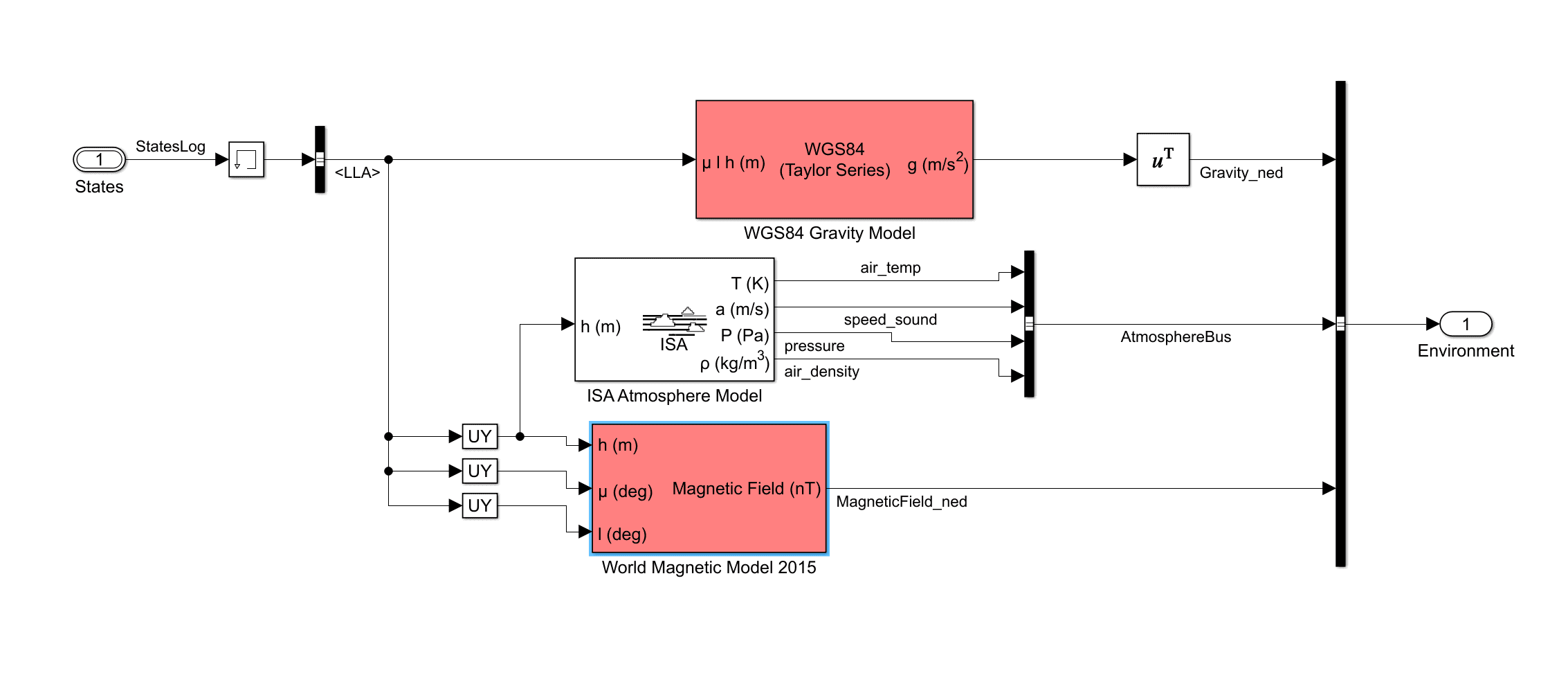
Environment Example Block
The static pressure sensor block can be easily derived by taking the pressure from the environment model. The only parameter that must be added is the temperature of the sensor (in this case is the OAT + 60):
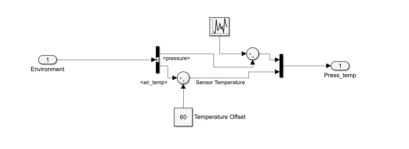
Static Pressure Example Block
The dynamic pressure input can be also obtained by using the standard dynamic pressure simulink block. The inputs are the speed (body axis) and the density:
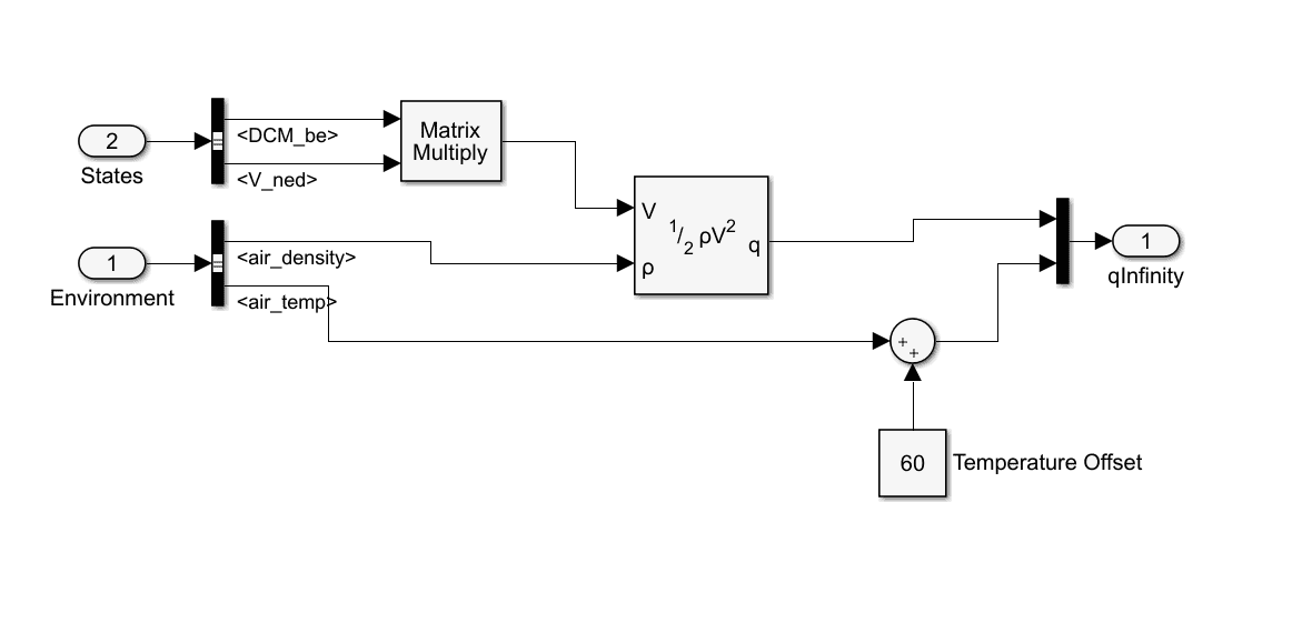
Dynamic Pressure Example Block
There is also a dedicated simulink block in the aerospace blockset that models a set of accelerometers and gyroscopes. The inputs of this block are the acceleration and angular velocities coming out of dynamics of the vehicle.
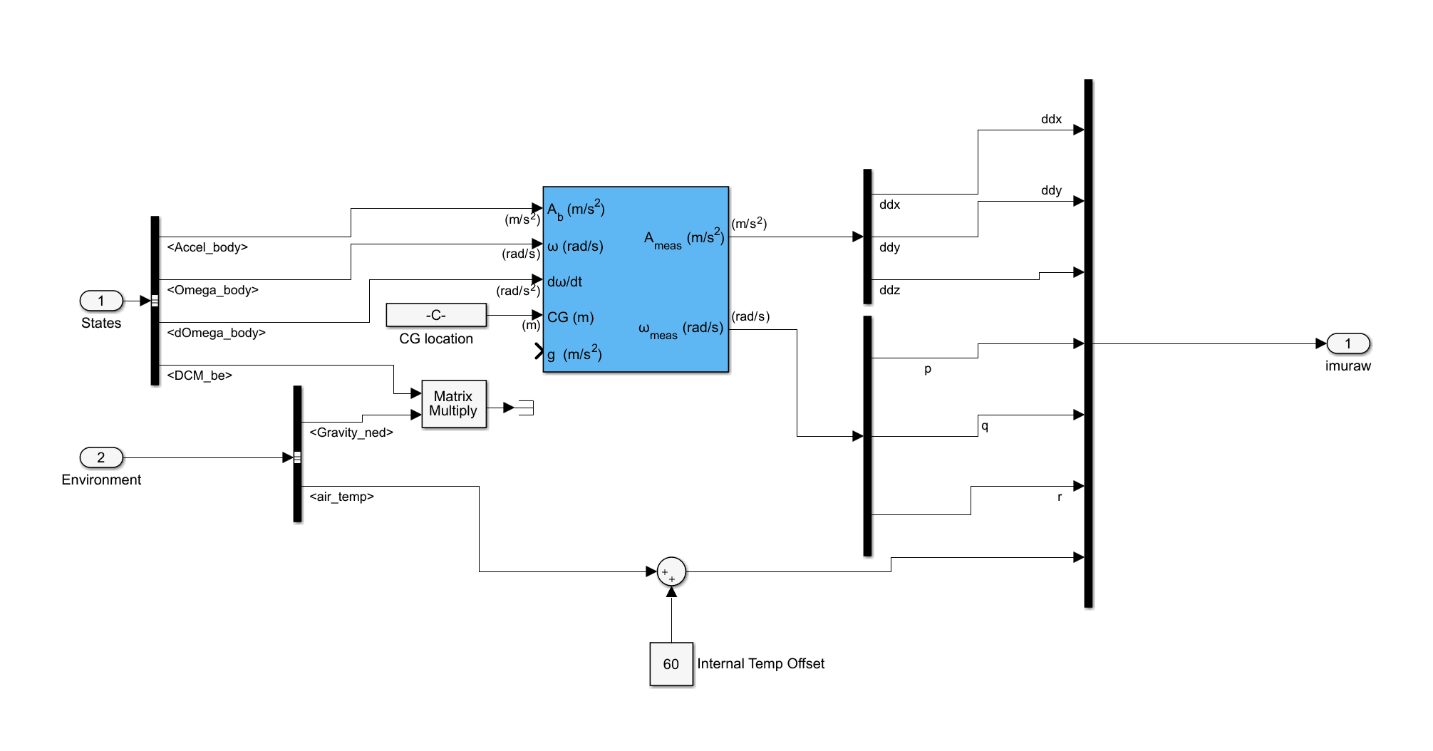
IMU Example Block
Warning
Do not connect the gravity port to the IMU block.
The magnetometer block is simply a rotated environment magnetic field where the temperature of sensor has been added (same as before OAT + 60). The reason why there is a selector crossing the signals is because there is a rotation matrix pre-configured in each PDI (the real magnetometer is not aligned with the autopilot axis):
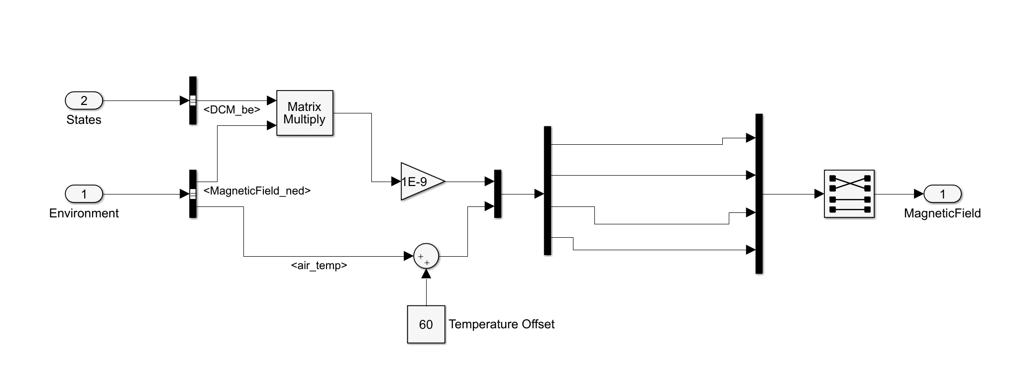
Magnetometer Example Block
The GNSS receiver and the relative position input (RTK) are only a multiplexor that creates an array. The position and the velocity are outputs of the vehicle model:
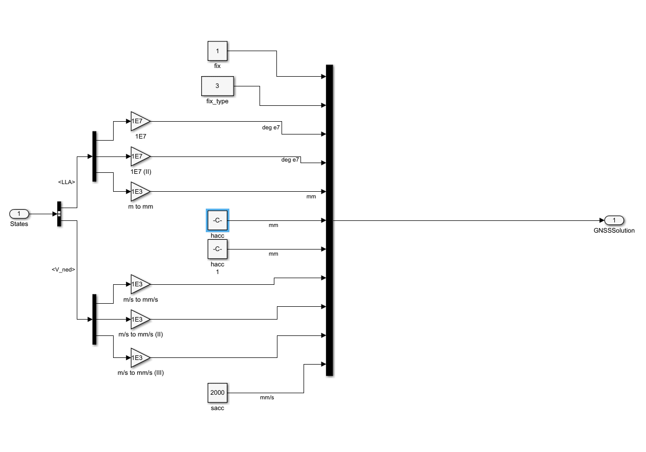
GNSS Receiver Example Block
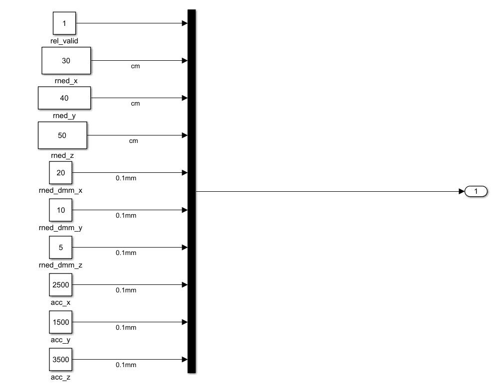
Relative Position (RTK) Example Block
The analogue inputs follow the same reasoning, the user must add the desired values to the mux:
ADCs Example Block
Veronte can manage input and output serial ports as explained :ref:`here <Device-Others-XPC-Uint8>`_. An easy way to create serial frames (data en length wires) is by using the simulink UDP block. Therefore, the data coming in to veronte should be sent though UDP (if this approach is taken):
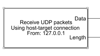
SCI Example Block
Monitoring Telemetry with Simulink
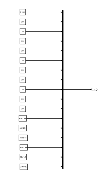
As explained before, there are three inputs specially dedicated to select custom telemetry (pins 22,23 and 24). The input structure of those is fixed and must be of size 50, as illustrasted here:
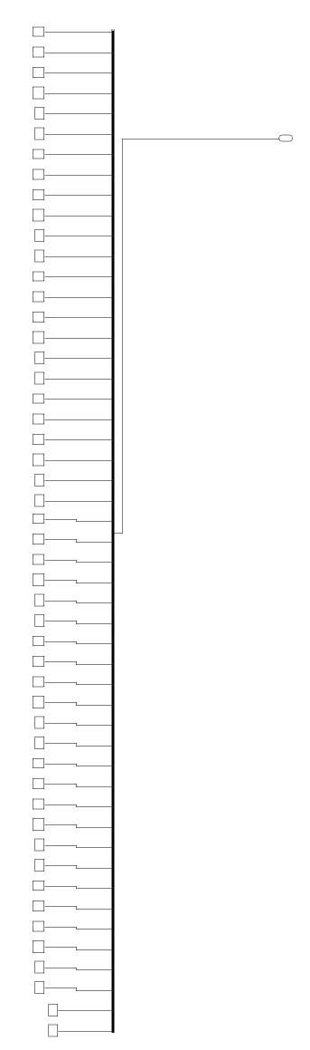
Telemetry ID Mux
The ID of each variable vailable in Veronte can be easily found in Veronte Pipe by adding a new workspace widget. The ID is labelled right before the variable name:
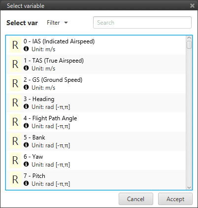
ID indicator
Lastly, to see their values, just place a scope connected to the matching output (pins 32, 33 or 34).
Complete Simulation
After setting the main blocks, the result should look like this:
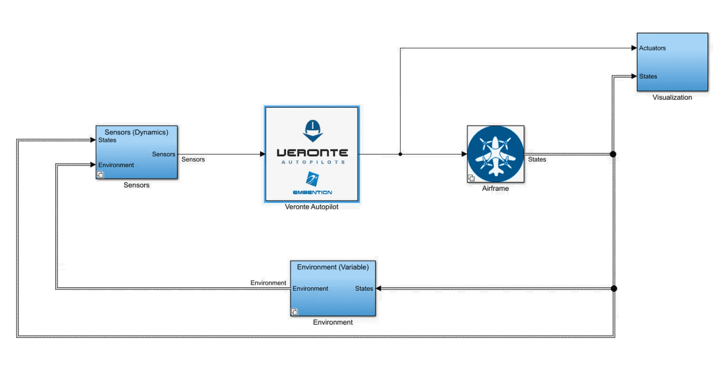
Complete Setup Example
The main systems are:
Veronte Autopilot: It contains our flight control software.
Airframe: a model of the flight dynamics.
Environment: a model of the atmosphere, magnetic field, WGS84…
Sensors: it contains individual blocks of all the sensors that veronte needs as input.
Visualization: It contains, scopes, flight instruments…
The time step should be set to 0.0002 as shown in the next figure in order to guarantee a good GNC/Adquisition frequency:
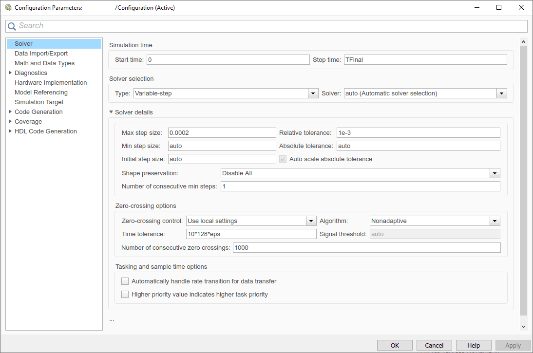
Time step settings
Connecting Simulink & Veronte Pipe
Our Software-in-the-loop simulator can be connected and used alonside Veronte Pipe software. To do it. Follow this steps:
Add a UDP serial communication block and connect it to USB data and length.
Add a second UDP serial communication block and connect it to the USB output of veronte.
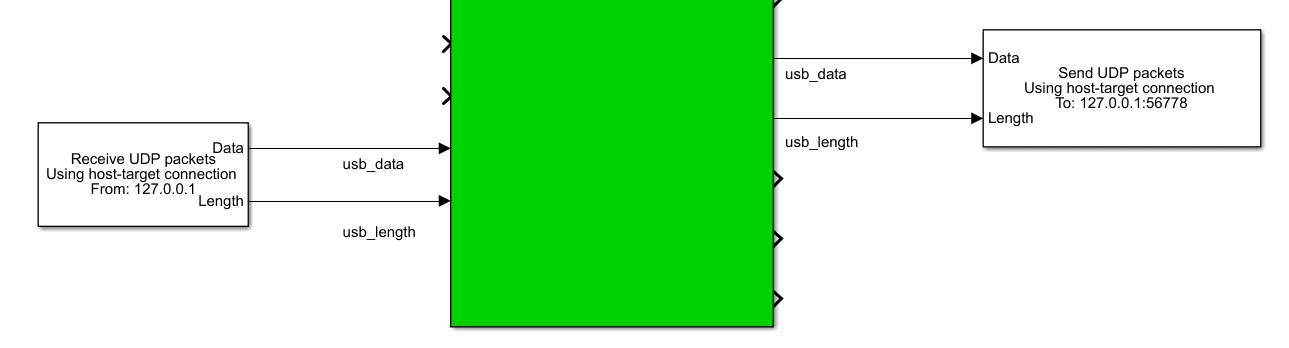
UDP Blocks
Configure your destination port.
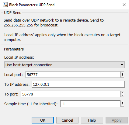
Destination UDP Port
Set an ethernet network in Preferences as shown using the destination port selected before.
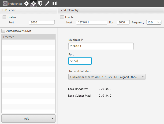
Destination UDP Port (Pipe)
Dealing with PDI files
PDI are uploaded exactly the same way that would be uploaded to a physical autopilot. Once connected to Veronte Pipe, a virtual autopilot will be detected in safe mode, then these steps can be followed.
Warning
Restart functionalities do no restart the simulation and must be done manually.
Veronte S-function deals with a direct copy of the binary files of a veronte autopilot, if a manual setup is needed, these files will be found in the same folder as the simulink block in a subfolder called mmc:
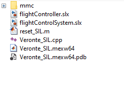
Folder structure (matlab)